3 Vector Calculus
3.0.1 Stoke’s Theorem
Let \(S\) be a piecewise smooth oriented surface in space, and let the boundary of \(S\) be a piecewise smooth simple closed curve \(C\). If \(\mathbf{F}(x, y, z)\) is a continuous vector function with continuous first partial derivatives in a domain containing \(S\), then:
\[\iint_S (\text{curl } \mathbf{F}) \cdot \mathbf{n} \, dA = \oint_C \mathbf{F} \cdot \mathbf{r}'(s) \, ds\].
In this formula:
- \(\mathbf{n}\) is the unit normal vector of \(S\).
- \(\mathbf{r}'(s)\) is the unit tangent vector of \(C\).
- \(s\) is the arc length of \(C\).
- The integration around \(C\) is performed in a sense consistent with the orientation of the normal vector \(\mathbf{n}\), following the right-hand rule.
3.0.3 Double Integral
The double integral is defined by the following identity: \[\iint_R f(x, y) \, dA = \lim_{m, n \to \infty} \sum_{i=1}^m \sum_{j=1}^n f(x_{ij}^*, y_{ij}^*) \Delta A\].
where * \(R\) is a closed bounded region in the \(xy\)-plane over which the function is integrated [1, 2]. * \(m\) and \(n\) are the number of subrectangles into which the region \(R\) is partitioned [3, 4]. * \(R_{ij}\) are the smaller subrectangles resulting from dividing \(R\) using a grid of lines parallel to the axes [4, 5]. * \(\Delta A\) represents the area of each subrectangle \(R_{ij}\) [4, 6]. * \((x_{ij}^*, y_{ij}^*)\) is an arbitrary sample point chosen within the subrectangle \(R_{ij}\) [4, 6]. * The limit is taken as \(m\) and \(n\) approach infinity such that the maximum diameter (the greatest distance between any two points within a subregion) approaches zero [3, 7]. * The function \(f(x, y)\), the integrand, is typically assumed to be continuous on \(R\) to ensure the limit exists and is independent of the choice of sample points [7, 8].
3.0.4 Double Integral Notational Variations
There exist double integral with two equivalent notations: * Differential Area Form: \(\displaystyle \iint_R f(x, y) \, dA\). * Coordinate Form: \(\displaystyle \iint_R f(x, y) \, dx \, dy\).
3.0.5 Projection
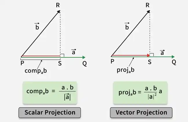
definition (vector projection) The vector representing the “shadow” of a vector \(\mathbf{b}\) cast onto the line containing a vector \(\mathbf{a}\), denoted by \(\text{proj}_{\mathbf{a}} \mathbf{b}\). Geometrically, it is the vector from the common initial point to the foot of the perpendicular dropped from the tip of \(\mathbf{b}\) onto the line containing \(\mathbf{a}\). It is calculated using the following formula:
- \(\text{proj}_{\mathbf{a}} \mathbf{b} = \left( \dfrac{\mathbf{a} \cdot \mathbf{b}}{|\mathbf{a}|^2} \right) \mathbf{a}\)
where
- \(\mathbf{a}, \mathbf{b}\) are vectors in a coordinate system.
- \(\mathbf{a} \cdot \mathbf{b}\) is the dot product of the two vectors.
- \(|\mathbf{a}|\) is the magnitude of vector \(\mathbf{a}\).
definition (scalar projection) The signed magnitude of the vector projection of \(\mathbf{b}\) onto \(\mathbf{a}\), also referred to as the component of \(\mathbf{b}\) along \(\mathbf{a}\), denoted by \(\text{comp}_{\mathbf{a}} \mathbf{b}\). It represents the length of the “shadow” and is positive if the angle between the vectors is acute and negative if it is obtuse. It is defined by the following formulas:
- \(\text{comp}_{\mathbf{a}} \mathbf{b} = \dfrac{\mathbf{a} \cdot \mathbf{b}}{|\mathbf{a}|}\)
- \(\text{comp}_{\mathbf{a}} \mathbf{b} = |\mathbf{b}| \cos \theta\)
where
- \(\mathbf{a}, \mathbf{b}\) are vectors in a coordinate system.
- \(\theta\) is the angle between vectors \(\mathbf{a}\) and \(\mathbf{b}\).
- \(|\mathbf{b}|\) is the magnitude of vector \(\mathbf{b}\).
3.0.6 Topology Reference
–> Topology.md